Compound interest is the interest that’s calculated both on the initial principal of a deposit or loan and on all previously accumulated interest. Professor Albert Einstein once said, “Compounding interest is the most powerful force in the universe.” It is doubtful whether Einstein really said that or not, but it doesn’t take away from the importance of the message. Compounding is a very powerful force that either works against you (borrowing) or for you (investing). In this article, I will show you how to use the compound interest formula in Excel. Let’s get started with the basics of compound interest.
Table of Contents Expand
Knowing Simple Interest Formula
You can use the simple interest formula to determine the amount of interest that will be charged on a sum of money at a certain rate and for a specified amount of time. The formula for determining simple interest is,
I = Pnr
Where,
- I = calculated simple interest
- P = Initial Principal
- n = number of periods
- r = annual interest rate
For example, if in 5 years you invest $100 at a rate of 5%. Then the calculated simple interest will be, I = $100*5/100*5, that is $25.
Knowing Compound Interest Formula
For calculating the future value of any investment earning at a constant rate of interest the following formula can be used. Which is,
Future Value = P*(1+r)^n
Where,
- P – the initial amount invested
- r – annual interest rate (as a decimal or a percentage)
- n – number of periods over which the investment is made
For example, if in 5 years you invest $100 at a rate of 5%. Then the calculated future value is, 100*(1+5%)^5 = 127.6282.
How to Use Compound Interest Formula in Excel: 4 Easy Ways
In this article, I will show you four easy ways to use the compound interest formula in Excel. In the first method, I will apply the basic formula of compound interest. Then, in the second procedure, I will calculate the compound interest for multiple years. Thirdly, I will consider different time contributions for calculating compound interest. Lastly, I will apply the FV function of Excel to calculate compound interest for different conditions.
For proceeding with our methods, I will use the following sample data set. Here, I have a table that states a $100 investment for 5 years at an annual interest rate of 5%.
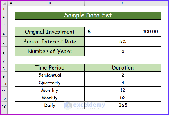
1. Applying Compound Interest Formula in Excel
In the first procedure, I will apply the basic formula of compound interest in Excel. Here we are going to calculate the future value of some ventures using the formula of compound interest in Excel. We can use the formula directly to calculate the future value in Excel. For that, follow the below-given steps.
Step 1:
- Firstly, write the following formula in cell C7.
=C4*(1+C5)^C6
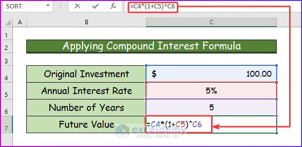
Step 2:
- Secondly, press Enter to see the future value in cell C7, which is $127.63.
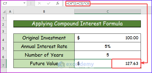
Read More: Methods to Apply Continuous Compound Interest Formula in Excel
2. Calculating Compound Interest Over Multiple Years
The future value of some amount of investment for a number of years can be shown using the same formula. Here the investment goes as the years add up. To learn more about this method, go through the following steps.
Step 1:
- Firstly, I will use the following data set for the following procedure.
- Here, I will calculate compound interest for each year separately.
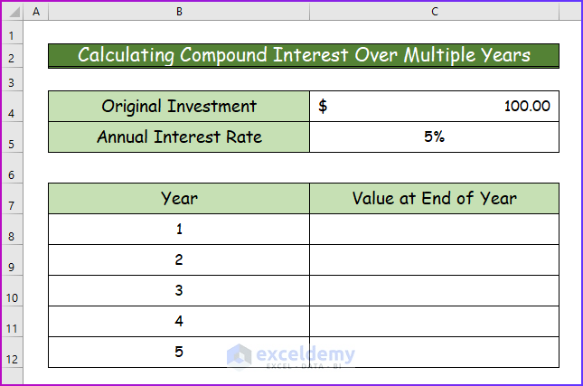
Step 2:
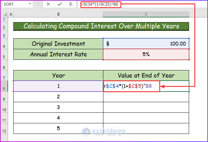
- Secondly, to do that, in cell C8, use the following formula.
=$C$4*(1+$C$5)^B8
- Here, I will absolute the values of cells C4 and C5 to use them in the lower columns also.
Step 3:
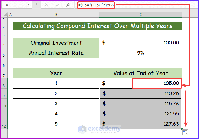
- Afterward, press Enter to see the desired interest for 1 year in cell C8, that is, $105.
- Then, use the AutoFill feature to drag the formula to the lower cells of that column.
Read More: Formula for Monthly Compound Interest in Excel
3. Determining Compound Interest with Time Contributions in Excel
In the third procedure, I will determine compound interest with different time contributions in Excel. From this method, you can calculate daily compound interest in Excel, as well as weekly, monthly, or semiannually. So, follow the below-given steps to learn the procedure.
Step 1:
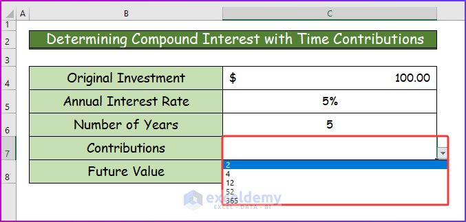
- First of all, I will create a dropdown to collect all the time contributions into one cell.
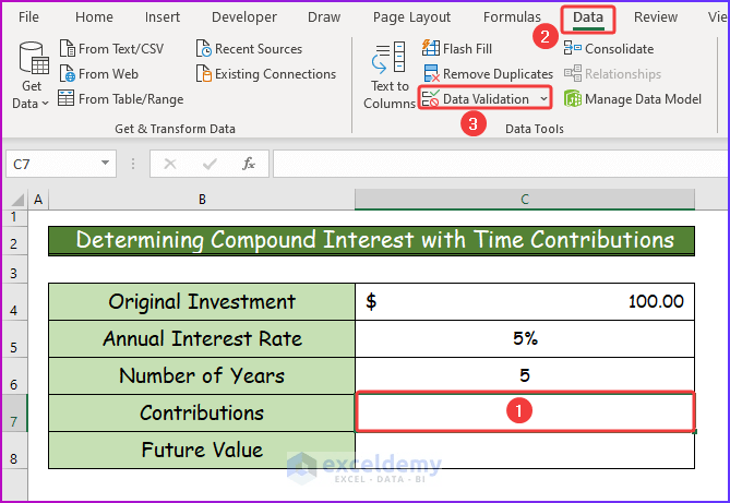
- For that, select cell C7 and then go to the Data tab of the ribbon.
- From there, in the Data Tools group, select Data Validation.
Step 2:
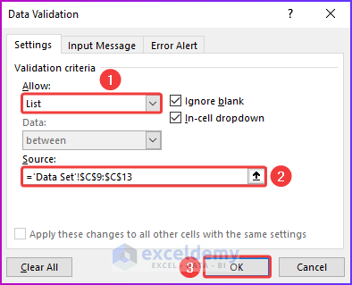
- Secondly, the Data Validation dialog box will appear.
- From there, under the Allow label, choose List.
- Then, in the Source type box, select the cell range C9:C13 from the Data Set worksheet that has the time interval of all the periods.
- Lastly, press OK.
Step 3:
- Thirdly, after performing the previous two steps, you will see the dropdown where all the time intervals are present.
Step 4:
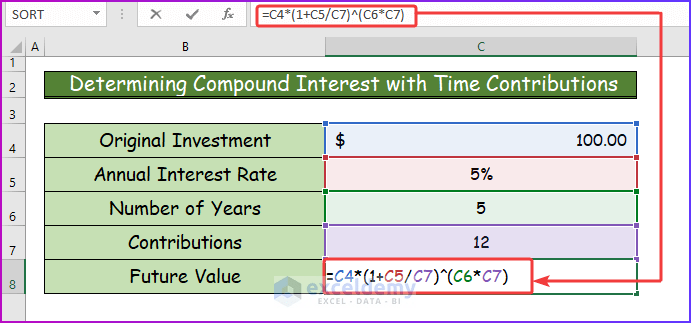
- Fourthly, insert the following formula in cell C8 to determine the compound interest for monthly contributions.
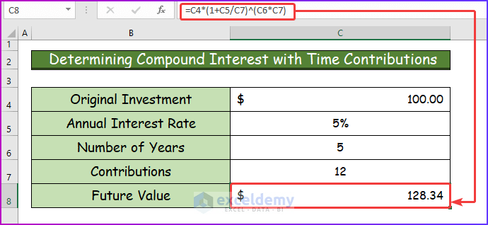
=C4*(1+C5/C7)^(C6*C7)
- For monthly contributions, the value of cell C7 will be 12.
Step 5:
- Finally, get the desired result by pressing Enter.
Step 6:
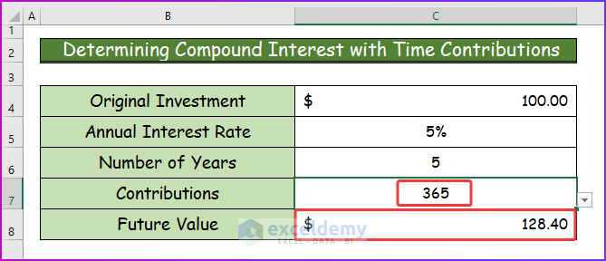
- Furthermore, by changing the cell value of C7 to 365, you can determine the compound interest with daily contributions.
- Hence, you can change C7 according to your preference.
Read More: How to Calculate Future Value When CAGR Is Known in Excel
4. Applying Excel FV Function for Calculating Compound Interest
It’s good practice to use Excel’s FV function, which calculates the future value based on different factors. The syntax for this FV function is,
FV(rate, nper, pmt, [pv], [type])
Where,
- rate -the interest rate
- nper -number of periods for the investment
- pmt -the periodic payment
- pv -the present value/initial investment
- type is optional.
4.1. Applying FV Function
In this section, I will show you the application of the FV function to calculate compound interest in Excel. Here, the application will be a simple one with no extra conditions. To apply this function, see the following steps.
Step 1:
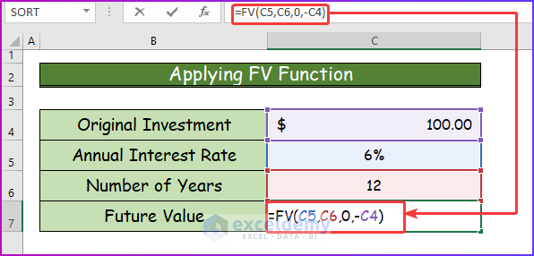
- First of all, write the following formula for the FV function in cell C7.
=FV(C5,C6,0,-C4)
- Here, 0 is used as there is no periodic payment.
- Also, I used the negative sign as Excel treats this as “money out” for your investment.
Step 2:
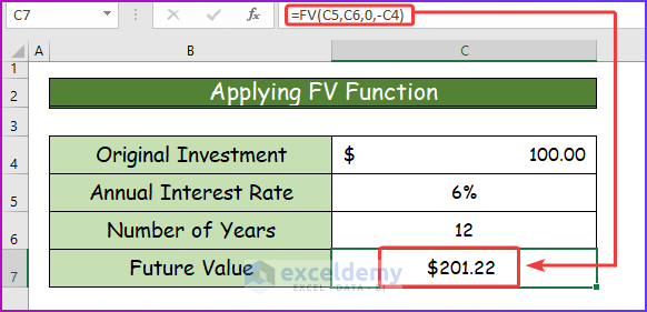
- Finally, after pressing Enter, you will see the desired compound interest of $201.22.
4.2. FV Function with Compounded Period
For calculating the future value to be compounded with a monthly, quarterly, weekly, or daily contribution, you need to divide the annual interest rate (for the FV function it is rate) with the contribution and multiply the contribution by the number of years (for the FV function it is nper).
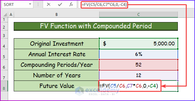
Let’s say we want to calculate the future value of the same factors. The only difference will be the compounding period. Here, the compounded periods will be the total number of weeks per year, which is 52. The steps below show how it is done.
Step 1:
- In the beginning, insert the following formula in cell C8 with compounding periods.
=FV(C5/C6,C7*C6,0,-C4)
Step 2:
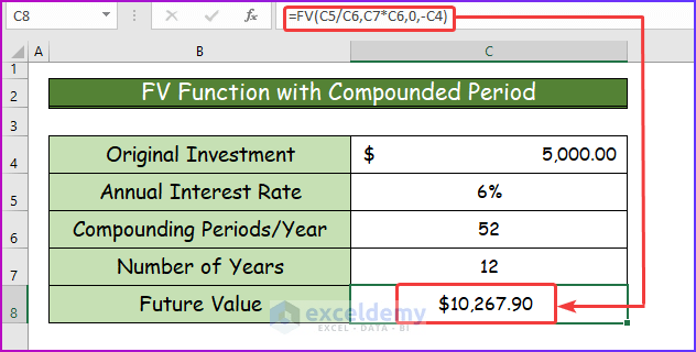
- Secondly, you will get the desired result by pressing Enter.
4.3. FV Function with Periodic Payment
Let’s calculate the compound interest with more options where additional contributions (pmet & type) are added. We will calculate the same example where an additional contribution of $500 is added. For doing this, see the following steps.
Step 1:
- Firstly, enter the following formula containing periodic payment in cell C10.
=FV(C5/C6,C7*C6,-C8,-C4,C9)
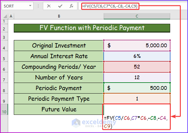
Step 2:
- Finally, after pressing Enter, you will get the desired result for this condition, which is $467,346.31.
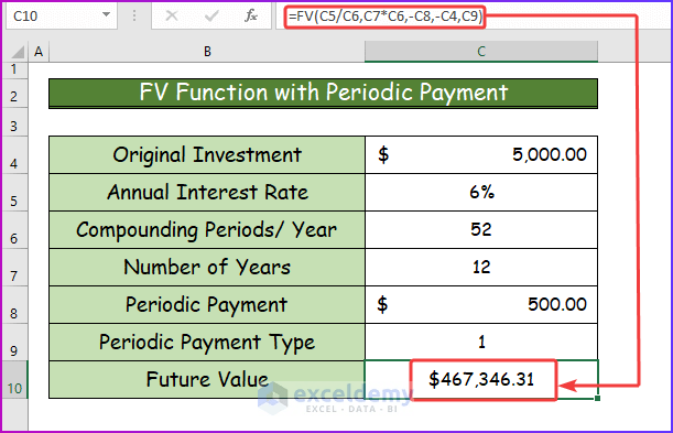
Read More: Excel Formula to Calculate Average Annual Compound Growth Rate
Calculating Compound Interest Between Two Dates in Excel
Sometimes, users have to calculate compound interest that is between two dates. Doing this calculation manually can be time-consuming and tiresome. By using the IPMT function of Excel, we can solve it easily. Suppose, We have to calculate the interest on a $5000 loan amount with monthly compounding and an interest rate of 6%. We are to find the interest between 15-Jun-2022 and 14-Jul-2022. The loan is to be repaid in 12 years. To do this type of calculation, see the following result.
Step 1:
- Firstly, type the following formula of the IPMT function in cell C11 to get the result.
=IPMT(C5/12,1,C7*C6,-C4)
- Here, 1 stands for the time interval between the two aforementioned dates, which is 1 month.
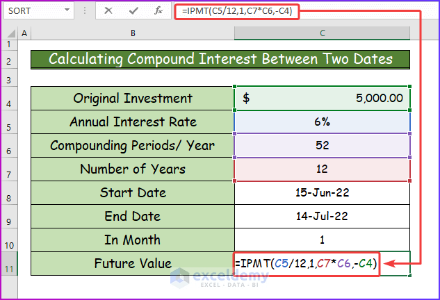
Step 2:
- Finally, by pressing Enter, you get the result for this procedure.
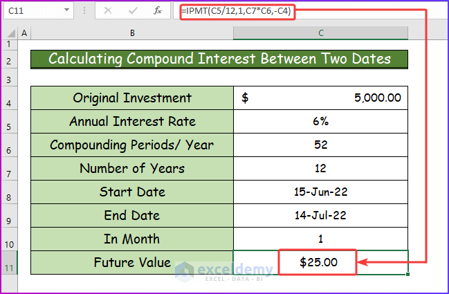
Determining Compound Interest with Regular Deposits
In this section, I will show you how to calculate compound interest using the Excel formula with regular deposits. To do this, we will use the Excel FV function. To learn more about this procedure, see the following steps.
Step 1:
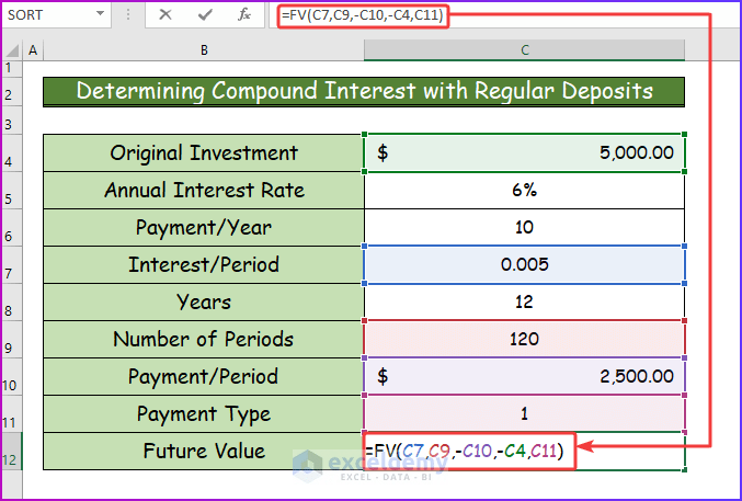
- At the beginning, insert the following formula of the FV function in cell C12 with all the necessary arguments.
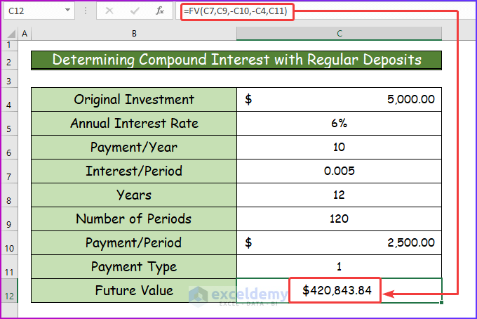
=FV(C7,C9,-C10,-C4,C11)
- Here, in cell C12, I select the payment type as 1.
- Also, we will also pay $2,500 ten times a year, which is a regular deposit.
Step 2:
- Finally, to get the desired result, press Enter after inserting the formula.
Read More: How to Calculate Compound Interest for Recurring Deposit in Excel
Download Practice Workbook
You can download the free Excel workbook here and practice on your own.
Compound Interest Formula.xlsx
Conclusion
That’s the end of this article. I hope you find this article helpful. After reading the above description, you will be able to use the compound interest formula in Excel. Please share any further queries or recommendations with us in the comments section below.
How to Use Compound Interest Formula in Excel: Knowledge Hub
- How to Calculate Compound Interest in Excel in Indian Rupees
- CAGR Formula in Excel: With Calculator and 7 Examples
- How to Calculate End Value from CAGR in Excel
- How to Calculate CAGR with Negative Number in Excel
- How to Calculate 3-Year CAGR with Formula in Excel
- How to Calculate 5 Year CAGR Using Excel Formula
- How to Create CAGR Graph in Excel
<< Go Back to Excel for Finance | Learn Excel